
Integrals can be difficult to solve, and can be exceptionally difficult to solve computationally. How do you program a way to solve an integral? There were many instances in calculus and differential equations courses I took that we could simply use an integral table. However, it does not make sense to program a whole mess of “if” statements, and there are other methods of programming, a simple solution is to approximate the integral. One thing computers are excellent at are iterating over an equation, therefore that is the most common way to calculate integrals on a computer.
A few days ago I was curious about how to approximate (really interpolate) integrals. I did some research and I decided to compare three common equations used to approximate, gaussian quadrature is much quicker, but I felt deserved its own post.
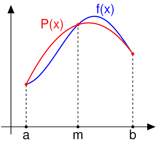
Midpoint Rule
From wikipedia:
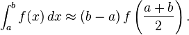
Where, given an equation such as sin(x), we approximate the integral over the points [a, b]. Given,
- a = 0
- b = π / 2
- f(x) = sin(x)
If we use the midpoint rule we get:
- (π / 2 – 0) * sin((π / 2 + 0) / 2) = (π / 2) * sin(π / 4)≈ 1.110720734
check for yourself via wolfram alpha
or

Now the actual solution to this is equal to 1,
meaning that the for error this approximation ≈ 11.07% (1.1107 / 1).
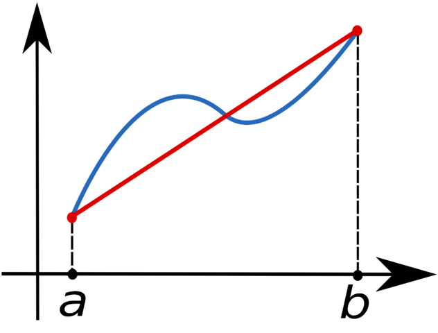
To improve this we use something called the composite midpoint rule. The composite midpoint rule is similar to the midpoint rule, except we split the equation into a number of separate smaller partitions which we iterate through. E.g. we take [a, b] and run the midpoint rule algorithm over smaller chunks, such as [a, t0], [t0, t1], [t1, b] or [0, π/6], [π /6, π/3], [π/3, π/2]. In this case we will approximate this integral as so:
- (π/6 – 0) * sin((π/6 + 0) / 2) ≈ 0.135517
- (π/3 – π/6) * sin((π/6 + π/3) / 2) ≈ 0.37024
- (π/2 – π/3) * sin((π/2 + π/3) / 2) ≈ 0.50575
- Total Combined: 0.135517 + 0.37024 + 0.50575 ≈ 1.0115
Since the solution to this integral is still equal to 1, our error using this approximation is ≈ 1.15% (1.0115 / 1).
OR
A ~9.92% reduction in error, by splitting the approximation into only 3 smaller partitions.
Approximations and Computations
Composite Midpoint Rule
Courtesy of Paul’s Online Math Notes
Since, we have computers who can perform millions of computations per second this makes approximations (such as the one above) quick and painless. Below is code which will generate 120 separate partitions for sin(x) over [0, π/2].
The output is: 1.00000713951
In other words, our error ~0.00071% (|1.00000713951 – 1| * 100).
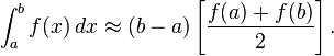
Composite Trapezoid Rule
Courtesy of Wikipedia:
With the following is the equation for the Trapezoidal Rule:
To increase accuracy, we create partitions and iterate over each of them.
The output is: 0.993440736
In other words, our error ~0.06559% (|0.993440736 – 1| * 100), slightly less accurate than the midpoint approach, but still very accurate.
Composite Simpson’s Rule
Courtesy of wikipedia:
With the following is the equation for the Simpson’s Rule:
![]()
Similar to previous approximation algorithms we increase accuracy, by creating partitions and iterating over each of them.
The output is: 1.0000
This gives an error of 0%, however if we look at iteration 121 as opposed to 120:
The output is: 0.987018942
This gives an error of ~1.2981% (|0.987018942 – 1| * 100)
Summary
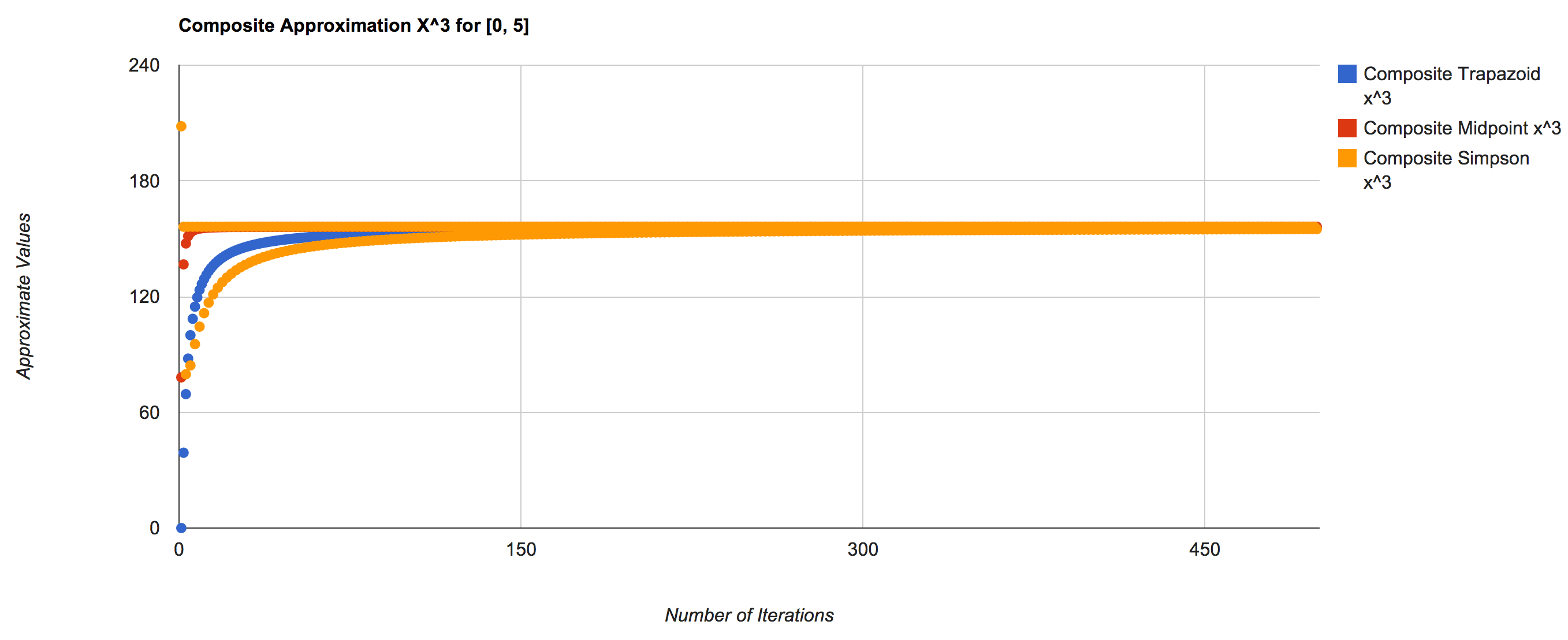
Integral approximations are important and useful while programming. Although they are not 100% accurate, the calculations are fast and the number of iterations required to approach the correct value (using these methods) is very quickly. The following are graphs to show just how quickly and the manner in which they approach the correct value:
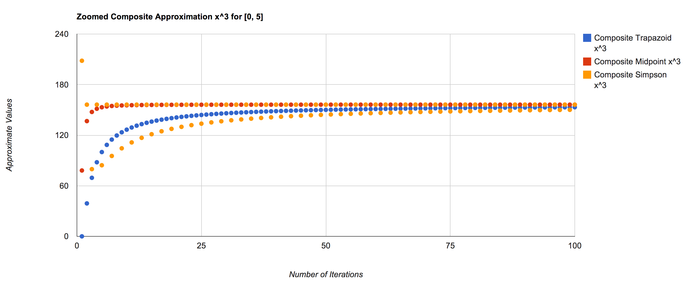
Integral of x^3 over [0, 5]:
And a closer view:
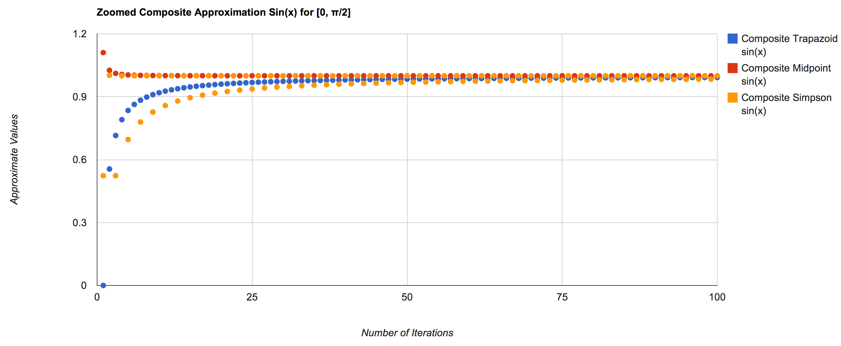
Integral of Sin(x) over [0, π/2]:
** This is the the same equation as the previous example.

A more zoomed in view:
The following code and data generated the graphs above:
Related Articles:
- Newtons Method and Fractals (austingwalters.com)
- Gaussian Quadrature (austingwalters.com)
- Introduction to Gauss-Legendre Quadrature (scientificpython.net)