
Linear Regression is defined as (from wikipedia):
An approach for modeling the relationship between a scalar dependent variable y and one or more explanatory variables denoted X. The case of one explanatory variable is called simple linear regression.
In this discussion we will be going over simple linear regression (meaning a linear/straight line). You may have seen this before on your graphic calculator or in high school. It is extremely useful for predicting trends, such as weights given height, heart rate given age, etc. Many people have used these functions in the past, but quite often it is a good idea to remind ourselves on how these methods are programed and applied in order to better understand how we can use them in the future. Linear regression is one of the most basic optimization problems, in which the error between the regression line and various points are calculated.
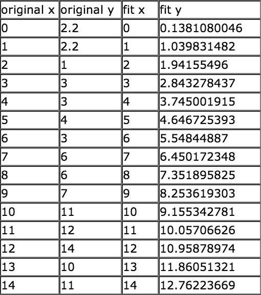
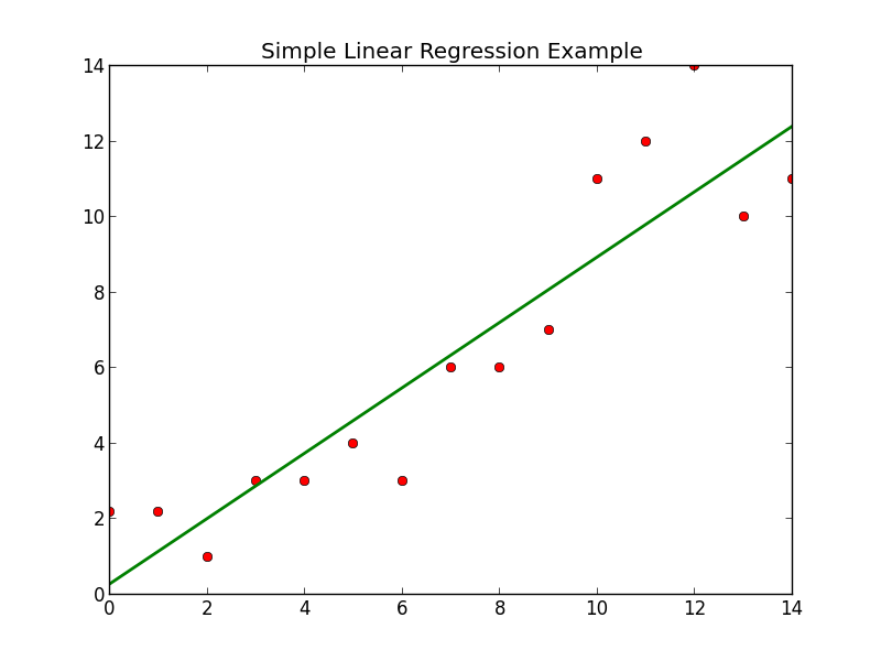
Without computation linear regression would be rather difficult, although simple to program it is very tedious to calculate by hand. Below is a table of various values, the original x and y are the various points, the fit x and y are the values that were obtained using a linear regression (the method will be described below):
As a plot:
Linear Regression Method
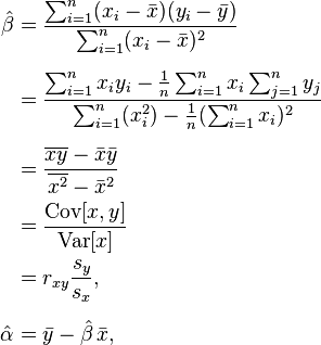
The equation that is used to calculate linear regression is as follows (from wikipedia):
Alright, so what does that mean?
Take the following image representing the differences between the points and the line obtained via linear regression above:
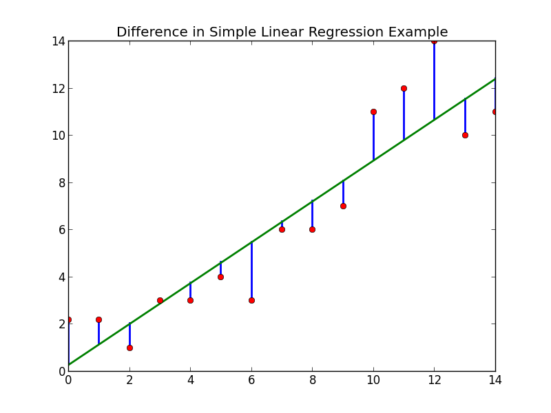
What we are attempting to do in linear regression is to minimize the sum of all of the blue lines. In other words find the line which is closest to all of the red points, by minimizing the sum of error between the each point and the linear regression line. With this more straight forward understanding, it is possible to rewrite the equation above in more laymen’s terms, which leaves you with the following (remember y = mx + b is the equation for a line):
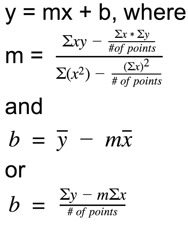 Where the sum represents the initial point to the final point (0 -> n so to speak), on which linear regression is going to be applied. If we look above this means x=0 to x=14. To me this equation seems far more straight forward and easy to understand.
This may seem overwhelming at first, but breaking it into chunks makes it much easier. If you are having trouble understanding try to break the problem into small chunks, also try to look at the programming example below.
Programming
Recall our equation:

If we were to program the above equation it would look as follows (in python):
The output is simply an array of various (x, y) points, for example if you fork from my github and run the program the output would be the images and table in this article.